Conformational ensembles generation, data representation and visualization of predicted flexibility properties using BioExcel Building Blocks (biobb) and FlexDyn tools

Workflow included in the ELIXIR 3D-Bioinfo Implementation Study:

Building on PDBe-KB to chart and characterize the conformation landscape of native proteins

This tutorial aims to illustrate the process of generating protein conformational ensembles from 3D structures and analysing its molecular flexibility, step by step, using the BioExcel Building Blocks library (biobb).

Conformational landscape of native proteins

Proteins are dynamic systems that adopt multiple conformational states, a property essential for many biological processes (e.g. binding other proteins, nucleic acids, small molecule ligands, or switching between functionaly active and inactive states). Characterizing the different conformational states of proteins and the transitions between them is therefore critical for gaining insight into their biological function and can help explain the effects of genetic variants in health and disease and the action of drugs.

Structural biology has become increasingly efficient in sampling the different conformational states of proteins. The PDB has currently archived more than 170,000 individual structures, but over two thirds of these structures represent multiple conformations of the same or related protein, observed in different crystal forms, when interacting with other proteins or other macromolecules, or upon binding small molecule ligands. Charting this conformational diversity across the PDB can therefore be employed to build a useful approximation of the conformational landscape of native proteins.

A number of resources and tools describing and characterizing various often complementary aspects of protein conformational diversity in known structures have been developed, notably by groups in Europe. These tools include algorithms with varying degree of sophistication, for aligning the 3D structures of individual protein chains or domains, of protein assemblies, and evaluating their degree of structural similarity. Using such tools one can align structures pairwise, compute the corresponding similarity matrix, and identify ensembles of structures/conformations with a defined similarity level that tend to recur in different PDB entries, an operation typically performed using clustering methods. Such workflows are at the basis of resources such as CATH, Contemplate, or PDBflex that offer access to conformational ensembles comprised of similar conformations clustered according to various criteria. Other types of tools focus on differences between protein conformations, identifying regions of proteins that undergo large collective displacements in different PDB entries, those that act as hinges or linkers, or regions that are inherently flexible.

To build a meaningful approximation of the conformational landscape of native proteins, the conformational ensembles (and the differences between them), identified on the basis of structural similarity/dissimilarity measures alone, need to be biophysically characterized. This may be approached at two different levels.

At the biological level, it is important to link observed conformational ensembles, to their functional roles by evaluating the correspondence with protein family classifications based on sequence information and functional annotations in public databases e.g. Uniprot, PDKe-Knowledge Base (KB). These links should provide valuable mechanistic insights into how the conformational and dynamic properties of proteins are exploited by evolution to regulate their biological function.
At the physical level one needs to introduce energetic consideration to evaluate the likelihood that the identified conformational ensembles represent conformational states that the protein (or domain under study) samples in isolation. Such evaluation is notoriously challenging and can only be roughly approximated by using computational methods to evaluate the extent to which the observed conformational ensembles can be reproduced by algorithms that simulate the dynamic behavior of protein systems. These algorithms include the computationally expensive classical molecular dynamics (MD) simulations to sample local thermal fluctuations but also faster more approximate methods such as Elastic Network Models and Normal Node Analysis (NMA) to model low energy collective motions. Alternatively, enhanced sampling molecular dynamics can be used to model complex types of conformational changes but at a very high computational cost.

The ELIXIR 3D-Bioinfo Implementation Study Building on PDBe-KB to chart and characterize the conformation landscape of native proteins focuses on:

Mapping the conformational diversity of proteins and their homologs across the PDB.
Characterize the different flexibility properties of protein regions, and link this information to sequence and functional annotation.
Benchmark computational methods that can predict a biophysical description of protein motions.

This notebook is part of the third objective, where a list of computational resources that are able to predict protein flexibility and conformational ensembles have been collected, evaluated, and integrated in reproducible and interoperable workflows using the BioExcel Building Blocks library. Note that the list is not meant to be exhaustive, it is built following the expertise of the implementation study partners.

The list of the selected tools is given in the following table, classified based on the underlying theoretical methods types, and presented together with the corresponding publication DOIs and URLs:

Tool	URL	Reference	Conda	Type
Concoord	URL	Reference	Conda	Atomistic intra-molecular interactions
ProDy	URL	Reference	Conda	Vibrational Analysis
FlexServ	URL	Reference	Conda	Vibrational Analysis, Coarse-Grained MD

NOLB	URL	Reference	Conda	Vibrational Analysis, Atomistic intra-molecular interactions
iMod	URL	Reference	Conda	Vibrational Analysis, Atomistic intra-molecular interactions

where the theoretical methods types are:

Vibrational analysis: Tools computing the vibrational normal modes of protein three-dimensional structures, taking as input PDB or mmCIF files. The movements associated with the vibrational modes (i.e. the eigenvectors) are known to be good descriptors of proteins dynamics, and of their flexibility. The type of output delivered by the different modes varies from protein motions to conformational ensembles.
Coarse-grained molecular simulations: Tools in this category make use of coarse-grained representations of the proteins and of molecular simulation techniques to generate conformational ensembles.
Atomistic intra-molecular interactions: Such tools make use of a potential to represent intra-molecular interactions and predict likely conformational changes in a protein structure.

The notebook is divided in two main blocks:

Conformational ensemble generation: where the different selected methods are used to build conformational ensembles that are then visualized using the NGL viewer.
Macromolecular flexibility analysis: where the generated ensembles are analysed to extract flexibility properties that will be used in subsequent comparisons with the conformational diversity and flexiblity observed in the PDB database.

Settings

Biobb modules used

biobb_flexserv: Tools to compute biomolecular flexibility on protein 3D structures.
biobb_flexdyn: Tools to study the conformational landscape of native proteins.
biobb_io: Tools to fetch biomolecular data from public databases.
biobb_structure_utils: Tools to modify or extract information from a PDB structure.
biobb_analysis: Tools to analyse Molecular Dynamics trajectories.
biobb_gromacs: Tools to setup and run Molecular Dynamics simulations with GROMACS MD package.

Auxiliary libraries used

jupyter: Free software, open standards, and web services for interactive computing across all programming languages.
plotly: Python interactive graphing library integrated in Jupyter notebooks.
nglview: Jupyter/IPython widget to interactively view molecular structures and trajectories in notebooks.
simpletraj: Lightweight coordinate-only trajectory reader based on code from GROMACS, MDAnalysis and VMD.
pandas: Open source data analysis and manipulation tool, built on top of the Python programming language.

Conda Installation and Launch

Take into account that, for this specific workflow, there are two environment files, one for linux OS and the other for mac OS:

linux

git clone https://github.com/bioexcel/biobb_wf_flexdyn.git
cd biobb_wf_flexdyn
conda env create -f conda_env/environment.linux.yml
conda activate biobb_wf_flexdyn
jupyter-notebook biobb_wf_flexdyn/notebooks/biobb_wf_flexdyn.ipynb

macos

git clone https://github.com/bioexcel/biobb_wf_flexdyn.git
cd biobb_wf_flexdyn
conda env create -f conda_env/environment.macos.yml
conda activate biobb_wf_flexdyn
jupyter-notebook biobb_wf_flexdyn/notebooks/biobb_wf_flexdyn.ipynb

Input parameters

Input parameters needed:

Auxiliary libraries: Libraries to be used in the workflow are imported once at the beginning
pdbCode: PDB code of the protein structure (e.g. 1AKE, https://doi.org/10.2210/pdb1AKE/pdb)

import os
import nglview
import simpletraj
import plotly
import plotly.graph_objs as go
import numpy as np
import pandas as pd
import ipywidgets
import json
import zipfile
from IPython.display import display, Markdown

pdbCode = "1ake"
num_frames = 300

Fetching PDB structure

Downloading PDB structure with the protein molecule from the RCSB PDB database.
Alternatively, a PDB file can be used as starting structure.

Building Blocks used:

Pdb from biobb_io.api.pdb

# Downloading desired PDB file 
# Import module
from biobb_io.api.pdb import pdb

# Create properties dict and inputs/outputs
downloaded_pdb = pdbCode+'.pdb'

prop = {
    'pdb_code': pdbCode,
    'api_id' : 'mmb'
}

#Create and launch bb
pdb(output_pdb_path=downloaded_pdb,
    properties=prop)

Selecting a model

If needed, select a single model from the PDB file.

Building Blocks used:

extract_model from biobb_structure_utils.utils.extract_model

from biobb_structure_utils.utils.extract_model import extract_model

pdb_model = pdbCode+'_model.pdb'

prop = {
    'models': [ 1 ]
}

extract_model(input_structure_path=downloaded_pdb,
              output_structure_path=pdb_model,
              properties=prop)

Selecting a monomer

If needed, select a single monomer (chain) from the PDB file.

Building Blocks used:

extract_chain from biobb_structure_utils.utils.extract_chain

from biobb_structure_utils.utils.extract_chain import extract_chain

monomer = pdbCode+'_monomer.pdb'

prop = {
    'chains': [ 'A' ]
}

extract_chain(input_structure_path=pdb_model,
            output_structure_path=monomer,
            properties=prop)

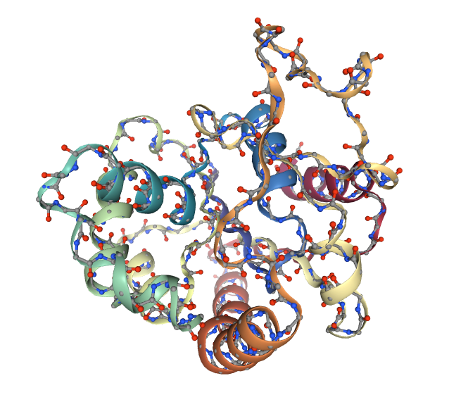
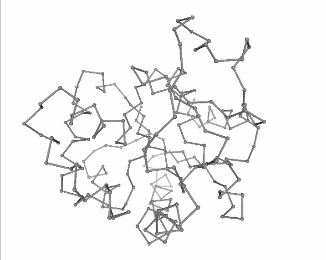
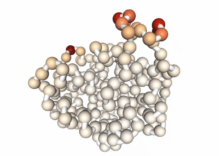
Visualizing the protein

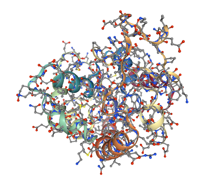
# Show protein
view = nglview.show_structure_file(monomer)
view.add_representation(repr_type='ball+stick', selection='all')
view._remote_call('setSize', target='Widget', args=['','600px'])
view

Generating the reduced (coarse-grained) structure (backbone)

Building Blocks used:

cpptraj_mask from biobb_analysis.ambertools.cpptraj_mask

from biobb_analysis.ambertools.cpptraj_mask import cpptraj_mask

prot_backbone = pdbCode + "_backbone.pdb"

prop = {
    'mask': 'backbone',
    'format': 'pdb'
}

cpptraj_mask(input_top_path=monomer,
            input_traj_path=monomer,
            output_cpptraj_path=prot_backbone,
            properties=prop)

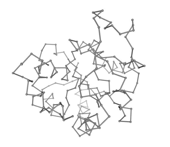
Visualizing the protein

# Show protein
view = nglview.show_structure_file(prot_backbone)
view.add_representation(repr_type='ball+stick', selection='all')
view._remote_call('setSize', target='Widget', args=['','600px'])
view

Generating the reduced (coarse-grained) structure (alpha carbons)

Building Blocks used:

cpptraj_mask from biobb_analysis.ambertools.cpptraj_mask

from biobb_analysis.ambertools.cpptraj_mask import cpptraj_mask

prot_ca = pdbCode + "_ca.pdb"

prop = {
    'mask': 'c-alpha',
    'format': 'pdb'
}

cpptraj_mask(input_top_path=monomer,
            input_traj_path=monomer,
            output_cpptraj_path=prot_ca,
            properties=prop)

Visualizing the protein

# Show protein
view = nglview.show_structure_file(prot_ca)
view.add_representation(repr_type='ball+stick', selection='all')
view.center()
view._remote_call('setSize', target='Widget', args=['','600px'])
view

Conformational Ensemble Generation

The next section is presenting a list of computational resources able to predict protein flexibility and conformational ensembles (the list is not meant to be exhaustive).

The notebook is intended to give an overview of the tools and resources considered relevant for the implementation study, namely tools that can be used to generate or characterize conformational ensembles of proteins.

CONCOORD

CONCOORD is a method to generate protein conformations around a known structure based on geometric restrictions. Principal component analyses of Molecular Dynamics (MD) simulations of proteins have indicated that collective degrees of freedom dominate protein conformational fluctuations. These large-scale collective motions have been shown essential to protein function in a number of cases. The notion that internal constraints and other configurational barriers restrict protein dynamics to a limited number of collective degrees of freedom has led to the design of the CONCOORD method to predict these modes without doing explicit, more CPU intensive, MD simulations.

The CONCOORD method consists of two stages: The first stage is the identification of all interatomic interactions in the starting structure. These interactions are divided among different categories, depending on the strength of the interaction. Covalent bonds form the tightest interactions and long-range non-bonded interactions are among the weakest interactions. Based on the strength of the interaction, a specific geometric freedom is given to each interacting pair. In this way, a set of upper and lower geometric bounds is obtained for all interacting pairs of atoms. The second stage consists of generating structures other than the starting structure that fulfill all geometric bounds. This is achieved by iteratively applying corrections to randomly generated coordinates untill all bounds are fulfilled.

References:

CONCOORD website: https://www3.mpibpc.mpg.de/groups/de_groot/concoord/concoord.html

Prediction of Protein Conformational Freedom From Distance Constraints.
Proteins, 1997, 29(2):240-51.
Available at: https://doi.org/10.1002/(sici)1097-0134(199710)29:2%3C240::aid-prot11%3E3.0.co;2-o

Building Blocks used:

concoord_dist from biobb_flexdyn.concoord.concoord_dist
concoord_disco from biobb_flexdyn.concoord.concoord_disco

from biobb_flexdyn.flexdyn.concoord_dist import concoord_dist

concoord_dist_pdb = pdbCode + "_dist.pdb"
concoord_dist_gro = pdbCode + "_dist.gro"
concoord_dist_dat = pdbCode + "_dist.dat"

concoord_lib = os.environ['CONDA_PREFIX']+"/share/concoord/lib"

prop = {
    'retain_hydrogens' : False,
    'cutoff' : 4.0,
    'env_vars_dict' : {
        'CONCOORD_OVERWRITE' : '1',
        'CONCOORDLIB' : concoord_lib
    }
}

concoord_dist(  input_structure_path=monomer,
                output_pdb_path=concoord_dist_pdb,
                output_gro_path=concoord_dist_gro,
                output_dat_path=concoord_dist_dat,
                properties=prop)

from biobb_flexdyn.flexdyn.concoord_disco import concoord_disco

concoord_disco_pdb = pdbCode + "_disco_traj.pdb"
concoord_disco_rmsd = pdbCode + "_disco_rmsd.dat"
concoord_disco_bfactor = pdbCode + "_disco_bfactor.pdb"

concoord_lib = os.environ['CONDA_PREFIX']+"/share/concoord/lib"

prop = {
    'vdw' : 4,
    'num_structs' : num_frames,
    'env_vars_dict' : {
        'CONCOORD_OVERWRITE' : '1',
        'CONCOORDLIB' : concoord_lib
    }
}

concoord_disco(     input_pdb_path=concoord_dist_pdb,
                    input_dat_path=concoord_dist_dat,
                    output_traj_path=concoord_disco_pdb,
                    output_rmsd_path=concoord_disco_rmsd,
                    output_bfactor_path=concoord_disco_bfactor,
                    properties=prop)

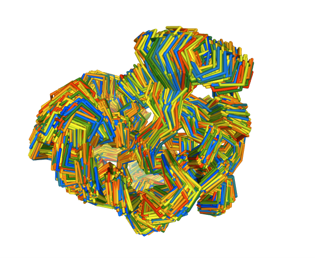
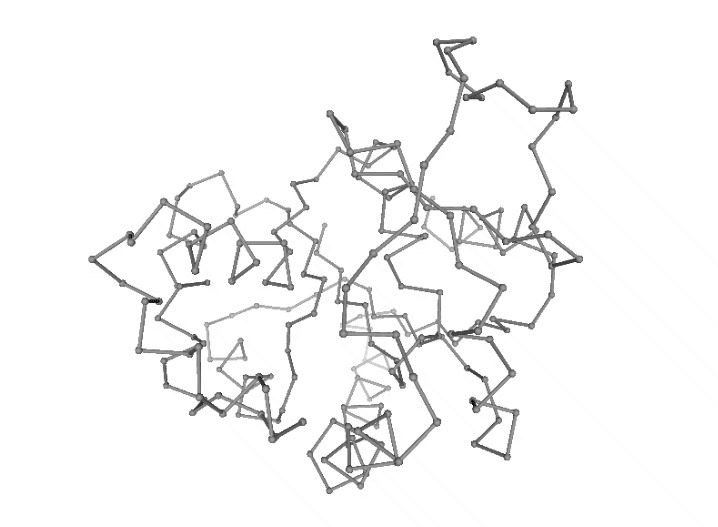
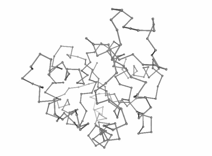
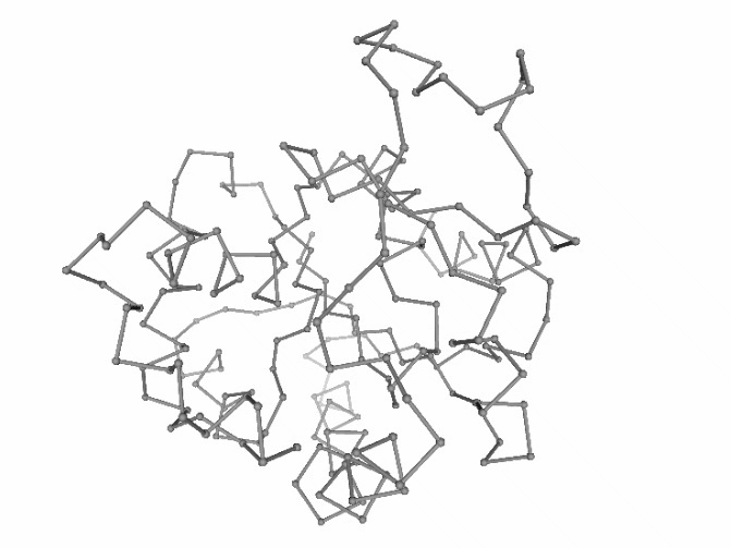
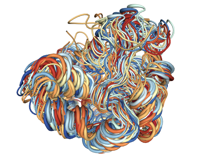
Visualizing the generated ensemble

# Show protein (if num_frames <= 100)

if (num_frames <= 100):
    view = nglview.show_structure_file(concoord_disco_pdb, default_representation=False)
    view.add_representation(repr_type='line', selection='all', color='modelindex')
    view.center()
    view._remote_call('setSize', target='Widget', args=['','600px'])
    view
else:
    #print("Visualizing a multi-model PDB with > 100 frames is highly dangerous. Please use the trajectory visualization below.")
    display(Markdown('<div class="alert alert-info">Visualizing a multi-model PDB with > 100 frames is highly dangerous. Please use the trajectory visualization below.</div>'))

    view = nglview.show_structure_file(concoord_disco_pdb, default_representation=False)
    view.clear_representations()
    view.add_representation(repr_type='backbone', selection='all', color='modelindex')
    view.center()
    view._remote_call('setSize', target='Widget', args=['','600px'])
    view

RMSd distribution of the generated ensemble

Building Blocks used:

cpptraj_rms from biobb_analysis.ambertools.cpptraj_rms

from biobb_analysis.ambertools.cpptraj_rms import cpptraj_rms

concoord_rmsd = pdbCode + "_concoord_rmsd.dat"

prop = {
    'start': 1,
    'end': -1,
    'steps': 1,
    'mask': 'c-alpha',
    'reference': 'experimental'
}
cpptraj_rms(input_top_path=concoord_dist_pdb,
            input_traj_path=concoord_disco_pdb,
            output_cpptraj_path=concoord_rmsd,
            input_exp_path= monomer,
            properties=prop)

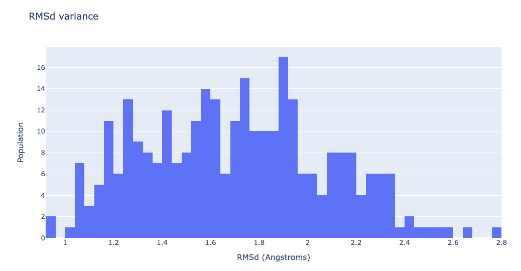
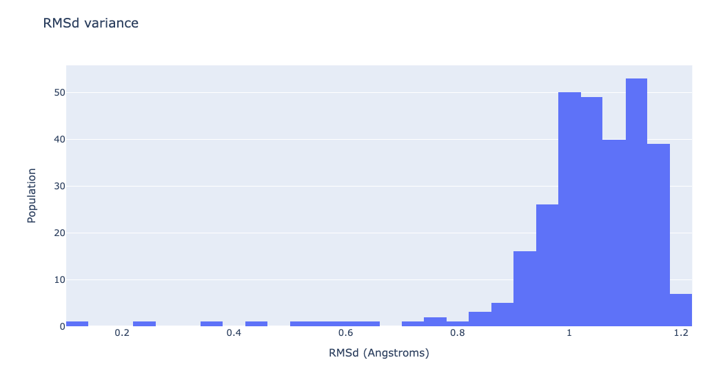
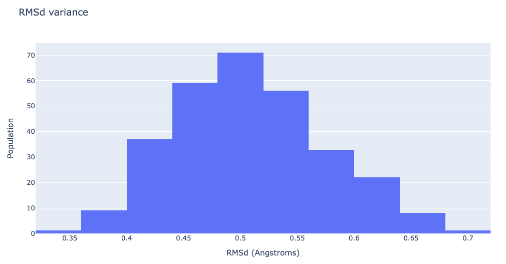
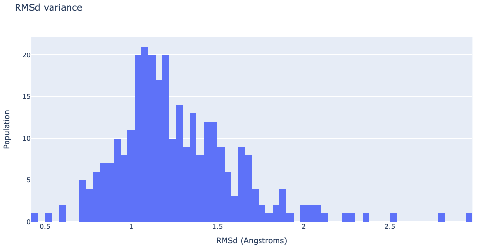
Visualizing the RMSd distribution

df = pd.read_csv(concoord_rmsd, header = 0, delimiter='\s+')

plotly.offline.init_notebook_mode(connected=True)

fig = {
    "data": [go.Histogram(x=df['RMSD_00004'], xbins=dict(
    size=0.04), autobinx=False)],
    "layout": go.Layout(title="RMSd variance",
                        xaxis=dict(title = "RMSd (Angstroms)"),
                        yaxis=dict(title = "Population")
                       )
}

plotly.offline.iplot(fig)

Converting the generated ensemble (for visualization purposes)

Building Blocks used:

cpptraj_convert from biobb_analysis.ambertools.cpptraj_convert

from biobb_analysis.ambertools.cpptraj_convert import cpptraj_convert

concoord_trr = pdbCode + "_disco_traj.trr"

prop = {
    'mask' : 'c-alpha',
    'format': 'trr'
}

cpptraj_convert(input_top_path=concoord_dist_pdb,
                input_traj_path=concoord_disco_pdb,
                output_cpptraj_path=concoord_trr,
                properties=prop)

Visualizing the generated ensemble (as a trajectory)

# Show trajectory
view = nglview.show_simpletraj(nglview.SimpletrajTrajectory(concoord_trr, prot_ca), gui=True)
view.center()
view.add_representation(repr_type='ball+stick', selection='all')
view._remote_call('setSize', target='Widget', args=['','600px'])
view

PRODY

ProDy is a free and open-source Python package for protein structural dynamics analysis. It is designed as a flexible and responsive API suitable for interactive usage and application development.

Structure analysis: ProDy has fast and flexible PDB and DCD file parsers, and powerful and customizable atom selections for contact identification, structure comparisons, and rapid implementation of new methods.
Dynamics analysis:
- Principal component analysis can be performed for:
  - heterogeneous X-ray structures (missing residues, mutations)
  - mixed structural datasets from Blast search
  - NMR models and MD snapshots (essential dynamics analysis)
- Normal mode analysis can be performed using:
  - Anisotropic network model (ANM)
  - Gaussian network model (GNM)
  - ANM/GNM with distance and property dependent force constants

References:

PRODY website: http://prody.csb.pitt.edu/

ProDy 2.0: Increased scale and scope after 10 years of protein dynamics modelling with Python.
Bioinformatics, 2021, 37(20):3657-3659.
Available at: https://doi.org/10.1093/bioinformatics/btab187

ProDy: Protein Dynamics Inferred from Theory and Experiments.
Bioinformatics, 2011, 27(11):1575-1577.
Available at: https://doi.org/10.1093/bioinformatics/btr168

Building Blocks used:

prody_anm from biobb_flexdyn.flexdyn.prody_anm

from biobb_flexdyn.flexdyn.prody_anm import prody_anm

prody_ensemble = pdbCode + "_prody_anm_traj.pdb"

prop = {
    'selection' : 'backbone',
    'num_structs' : num_frames,
    'rmsd' : 2.0
}

prody_anm(  input_pdb_path=monomer,
            output_pdb_path=prody_ensemble,
            properties=prop)

RMSd distribution of the generated ensemble

Building Blocks used:

cpptraj_rms from biobb_analysis.ambertools.cpptraj_rms

from biobb_analysis.ambertools.cpptraj_rms import cpptraj_rms

prody_rmsd = pdbCode + "_prody_rmsd.dat"

prop = {
    'start': 1,
    'end': -1,
    'steps': 1,
    'mask': 'c-alpha',
    'reference': 'experimental'
}
cpptraj_rms(input_top_path=prody_ensemble,
            input_traj_path=prody_ensemble,
            output_cpptraj_path=prody_rmsd,
            input_exp_path= monomer,
            properties=prop)

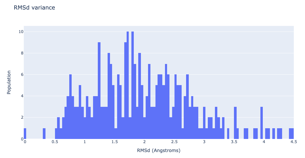
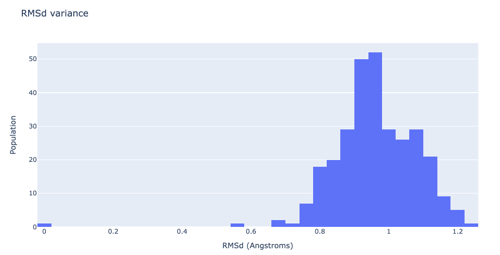
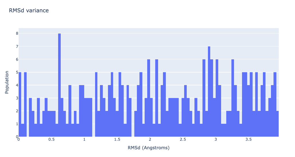
Visualizing the RMSd distribution

df = pd.read_csv(prody_rmsd, header = 0, delimiter='\s+')

plotly.offline.init_notebook_mode(connected=True)

fig = {
    "data": [go.Histogram(x=df['RMSD_00004'], xbins=dict(
    size=0.04), autobinx=False)],
    "layout": go.Layout(title="RMSd variance",
                        xaxis=dict(title = "RMSd (Angstroms)"),
                        yaxis=dict(title = "Population")
                       )
}

plotly.offline.iplot(fig)

Converting the generated ensemble (for visualization purposes)

Building Blocks used:

cpptraj_convert from biobb_analysis.ambertools.cpptraj_convert

from biobb_analysis.ambertools.cpptraj_convert import cpptraj_convert

prody_trr = pdbCode + "_prody_anm_traj.trr"

prop = {
    'mask' : 'c-alpha',
    'format': 'trr'
}

cpptraj_convert(input_top_path=prot_backbone,
                input_traj_path=prody_ensemble,
                output_cpptraj_path=prody_trr,
                properties=prop)

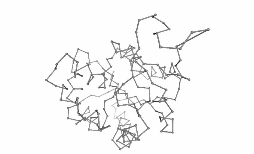
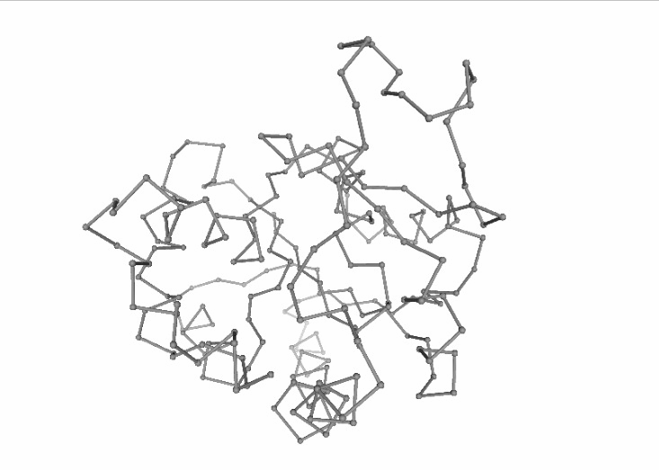
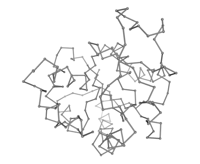
Visualizing the generated ensemble (as a trajectory)

# Show trajectory
view = nglview.show_simpletraj(nglview.SimpletrajTrajectory(prody_trr, prot_ca), gui=True)
view.center()
view.add_representation(repr_type='ball+stick', selection='all')
view._remote_call('setSize', target='Widget', args=['','600px'])
view

FLEXSERV

Despite recent advances in experimental techniques, the study of molecular flexibility is mostly a task for theoretical methods. The most powerful of them is atomistic molecular dynamics (MD), a rigorous method with solid physical foundations, which provides accurate representations of protein flexibility under physiological-like environments. Unfortunately, despite its power, MD is a complex technique, computationally expensive and their use requires a certain degree of expertise. The alternative to atomistic MD is the use of coarse-grained methods coupled to simple potentials. By using these techniques we assume a lost of atomic detail to gain formal and computational simplicity in the representation of near-native state flexibility of proteins. Unfortunately, despite its power, the practical use of coarse-grained methods is still limited, due mostly to the lack of standardized protocols for analysis and the existence of a myriad of different algorithms distributed in different websites.

FlexServ webserver and associated BioBB module integrate three coarse-grained algorithms for the representation of protein flexibility:

i) Brownian dynamics (BD)
ii) Discrete dynamics (DMD)
iii) Normal mode analysis (NMA) based on different types of elastic networks

This next cells of this tutorial show how to extract molecular flexibility (conformational ensemble) from a single, static structure downloaded from the PDB database, generating its coarse-grained, reduced representation ($C_{\alpha}$) and running the previously mentioned coarse-grained algorithms.

References:

FLEXSERV website: https://mmb.irbbarcelona.org/FlexServ/

FlexServ: an integrated tool for the analysis of protein flexibility.
Bioinformatics, Volume 25, Issue 13, 2009, Pages 1709–1710,.
Available at: https://doi.org/10.1093/bioinformatics/btp304

Building Blocks used:

bd_run from biobb_flexserv.flexserv.bd_run
dmd_run from biobb_flexserv.flexserv.dmd_run
nma_run from biobb_flexserv.flexserv.nma_run

Brownian Dynamics (BD)

The Brownian Dynamics (BD) method introduces the protein in an stochastic bath that keeps the temperature constant and modulates the otherwise extreme oscillations of the residues. This bath is simulated with two terms accounting for a velocity-dependent friction and stochastic forces due to the solvent environment. Velocity Verlet algorithm is used to solve the stochastic differential equation (equation of motion) for alpha-carbons ($C\alpha$). The equation of motion is integrated using Verlet’s algorithm The potential energy used to compute forces in the equation of motion assumes a coarse-grained representation of the protein ($C\alpha$-only) and a quasi-harmonic representation of the interactions (similar to that suggested by Kovacs et al. 2004).

The initial condition is a native structure (or MD-averaged conformation) that is supposed to be in the minimal energy state, from which the relative vectors are computed. Brownian Dynamics (BD) simulation time scales were equivalent to those considered in Molecular Dynamics (MD).

Reference:
Exploring the Suitability of Coarse-Grained Techniques for the Representation of Protein Dynamics.
Biophysical Journal, Volume 95, Issue 5, 1 September 2008, Pages 2127-2138
Available at: https://doi.org/10.1529/biophysj.107.119115

# Running Brownian Dynamics (BD)
# Import module
from biobb_flexserv.flexserv.bd_run import bd_run

# Create properties dict and inputs/outputs

bd_log = pdbCode + '_flexserv_bd_ensemble.log'
bd_crd = pdbCode + '_flexserv_bd_ensemble.mdcrd'

wfreq = 100
time = num_frames * wfreq

prop = {
    'time': time,
    'wfreq': wfreq
}

bd_run( 
     input_pdb_path=prot_ca,
     output_crd_path=bd_crd,
     output_log_path=bd_log,
     properties=prop
)

RMSd distribution of the generated ensemble

Building Blocks used:

cpptraj_rms from biobb_analysis.ambertools.cpptraj_rms

from biobb_analysis.ambertools.cpptraj_rms import cpptraj_rms

flexserv_bd_rmsd = pdbCode + "_flexserv_bd_rmsd.dat"

prop = {
    'start': 1,
    'end': -1,
    'steps': 1,
    'mask': 'c-alpha',
    'reference': 'experimental'
}
cpptraj_rms(input_top_path=prot_ca,
            input_traj_path=bd_crd,
            output_cpptraj_path=flexserv_bd_rmsd,
            input_exp_path=monomer,
            properties=prop)

Visualizing the RMSd distribution

df = pd.read_csv(flexserv_bd_rmsd, header = 0, delimiter='\s+')

plotly.offline.init_notebook_mode(connected=True)

fig = {
    "data": [go.Histogram(x=df['RMSD_00004'], xbins=dict(
    size=0.04), autobinx=False)],
    "layout": go.Layout(title="RMSd variance",
                        xaxis=dict(title = "RMSd (Angstroms)"),
                        yaxis=dict(title = "Population")
                       )
}

plotly.offline.iplot(fig)

Fitting and converting the generated ensemble (for visualization purposes)

Building Blocks used:

cpptraj_rms from biobb_analysis.ambertools.cpptraj_rms

from biobb_analysis.ambertools.cpptraj_rms import cpptraj_rms

flexserv_bd_rmsd = pdbCode + "_flexserv_bd_rmsd.dat" 
flexserv_bd_traj_fitted = pdbCode + "_flexserv_bd_traj_fitted.trr"

prop = {
    'start': 1,
    'end': -1,
    'steps': 1,
    'mask': 'c-alpha',
    'reference': 'experimental'
}
cpptraj_rms(input_top_path=prot_ca,
            input_traj_path=bd_crd,
            output_cpptraj_path=flexserv_bd_rmsd,
            output_traj_path=flexserv_bd_traj_fitted,
            input_exp_path= monomer,
            properties=prop)

Visualizing the generated ensemble (as a trajectory)

# Show trajectory
view = nglview.show_simpletraj(nglview.SimpletrajTrajectory(flexserv_bd_traj_fitted, prot_ca), gui=True)
view.add_representation(repr_type='ball+stick', selection='all')
view.center()
view._remote_call('setSize', target='Widget', args=['','600px'])
view

Discrete Molecular Dynamics (DMD)

With the Discrete Molecular Dynamics (DMD) method, the proteins are modelled as a system of beads ($C\alpha$ atoms) interacting through a discontinuous potential (square wells in the used tool). Outside the discontinuities, potentials are considered constant, thereby implying a ballistic regime for the particles (constant potential, constant velocity) in all conditions, except at such time as when the particles reach a potential discontinuity (this is called “an event” or “a collision”). At this time, the velocities of the colliding particles are modified by imposing conservation of the linear momentum, angular momentum, and total energy. Since the particles were constrained to move within a configurational space where the potential energy is constant (infinite square wells), the kinetic energy remains unchanged and therefore all collisions are assumed to be elastic.

DMD has a major advantage over techniques like MD because, as it does not require the integration of the equations of motion at fixed time steps, the calculation progresses from event to event. In practice, the time between events decreases with temperature and density and depends on the number of particles N. The equation of motion, corresponding to constant velocity, is solved analytically.

As the integration of Newton’s equations is no longer the rate limiting step, calculations can be extended for very long simulation periods and large systems, provided an efficient algorithm for predicting collisions is used.

The collision between particles i and j is associated with a transfer of linear momentum in the direction of the vector $\vec{r_{ij}}$. To calculate the change in velocities, the velocity of each particle is projected in the direction of the vector $\vec{r_{ij}}$ so that the conservation equations become one-dimensional along the interatomic coordinate.

# Running Discrete Molecular Dynamics (DMD)
# Import module
from biobb_flexserv.flexserv.dmd_run import dmd_run

# Create properties dict and inputs/outputs

dmd_log = pdbCode + '_flexserv_dmd_ensemble.log'
dmd_crd = pdbCode + '_flexserv_dmd_ensemble.mdcrd'

prop = {
    'frames': num_frames
}
dmd_run( 
     input_pdb_path=prot_ca,
     output_crd_path=dmd_crd,
     output_log_path=dmd_log,
     properties=prop
)

RMSd distribution of the generated ensemble

Building Blocks used:

cpptraj_rms from biobb_analysis.ambertools.cpptraj_rms

from biobb_analysis.ambertools.cpptraj_rms import cpptraj_rms

flexserv_dmd_rmsd = pdbCode + "_flexserv_dmd_rmsd.dat"

prop = {
    'start': 1,
    'end': -1,
    'steps': 1,
    'mask': 'c-alpha',
    'reference': 'experimental'
}

cpptraj_rms(input_top_path=prot_ca,
            input_traj_path=dmd_crd,
            output_cpptraj_path=flexserv_dmd_rmsd,
            input_exp_path= monomer,
            properties=prop)

Visualizing the RMSd distribution

df = pd.read_csv(flexserv_dmd_rmsd, header = 0, delimiter='\s+')

plotly.offline.init_notebook_mode(connected=True)

fig = {
    "data": [go.Histogram(x=df['RMSD_00004'], xbins=dict(
    size=0.04), autobinx=False)],
    "layout": go.Layout(title="RMSd variance",
                        xaxis=dict(title = "RMSd (Angstroms)"),
                        yaxis=dict(title = "Population")
                       )
}

plotly.offline.iplot(fig)

Fitting and converting the generated ensemble (for visualization purposes)

Building Blocks used:

cpptraj_rms from biobb_analysis.ambertools.cpptraj_rms

from biobb_analysis.ambertools.cpptraj_rms import cpptraj_rms

flexserv_dmd_rmsd = pdbCode + "_flexserv_dmd_rmsd.dat"
flexserv_dmd_traj_fitted = pdbCode + "_flexserv_dmd_traj_fitted.trr"

prop = {
    'start': 1,
    'end': -1,
    'steps': 1,
    'mask': 'c-alpha',
    'reference': 'experimental'
}

cpptraj_rms(input_top_path=prot_ca,
            input_traj_path=dmd_crd,
            output_cpptraj_path=flexserv_dmd_rmsd,
            output_traj_path=flexserv_dmd_traj_fitted,
            input_exp_path= monomer,
            properties=prop)

Visualizing the generated ensemble (as a trajectory)

# Show trajectory
view = nglview.show_simpletraj(nglview.SimpletrajTrajectory(flexserv_dmd_traj_fitted, prot_ca), gui=True)
view.add_representation(repr_type='ball+stick', selection='all')
view.center()
view._remote_call('setSize', target='Widget', args=['','600px'])
view

Normal Mode Analysis (NMA)

Normal Mode Analysis (NMA) can be defined as the multidimensional treatment of coupled oscillators from the analysis of force-derivatives in equilibrium conformations. This methodology assumes that the displacement of an atom from its equilibrium position is small and that the potential energy in the vicinity of the equilibrium position can be approximated as a sum of terms that are quadratic in the atomic displacements. In its purest form, it uses the same all-atom force field from a MD simulation, implying a prior in vacuo minimization (Go and Scheraga 1976; Brooks III, Karplus et al. 1987).

Tirion (1996) proposed a simplified model where the interaction between two atoms was described by Hookean pairwise potential where the distances are taken to be at the minimum, avoiding the minimization (referred as Elastic Network Model -ENM-). This idea being further extended to use coarse-grained ($C\alpha$) protein representation by several research groups, as in the Gaussian Network Model -GNM- (Bahar et al. 1997; Haliloglu et al. 1997). The GNM model was later extended to a 3-D, vectorial Anisotropic Network Model -ANM-, which is the formalism implemented in the following cell (Atilgan et al. 2001). Through the diagonalization of the hessian matrix, the ANM provides eigenvalues and eigenvectors that not only describe the frequencies and shapes of the normal modes, but also their directions.

Once NMA is performed and the set of eigenvectors/eigenvalues is determined, Cartesian pseudo-trajectories at physiologic temperature can be obtained by activating normal mode deformations using a Metropolis Monte Carlo algorithm. The displacements obtained by such algorithm can then be projected to the Cartesian space to generate the pseudo-trajectories.

# Running Normal Mode Analysis (NMA)
# Import module
from biobb_flexserv.flexserv.nma_run import nma_run

# Create properties dict and inputs/outputs

nma_log = pdbCode + '_flexserv_nma_ensemble.log'
nma_crd = pdbCode + '_flexserv_nma_ensemble.mdcrd'

prop = {
    'frames' : num_frames
}

nma_run( 
     input_pdb_path=prot_ca,
     output_crd_path=nma_crd,
     output_log_path=nma_log,
     properties=prop
)

RMSd distribution of the generated ensemble

Building Blocks used:

cpptraj_rms from biobb_analysis.ambertools.cpptraj_rms

from biobb_analysis.ambertools.cpptraj_rms import cpptraj_rms

flexserv_nma_rmsd = pdbCode + "_flexserv_nma_rmsd.dat"

prop = {
    'start': 1,
    'end': -1,
    'steps': 1,
    'mask': 'c-alpha',
    'reference': 'experimental'
}

cpptraj_rms(input_top_path=prot_ca,
            input_traj_path=nma_crd,
            output_cpptraj_path=flexserv_nma_rmsd,
            input_exp_path= monomer,
            properties=prop)

Visualizing the RMSd distribution

df = pd.read_csv(flexserv_nma_rmsd, header = 0, delimiter='\s+')

plotly.offline.init_notebook_mode(connected=True)

fig = {
    "data": [go.Histogram(x=df['RMSD_00004'], xbins=dict(
    size=0.04), autobinx=False)],
    "layout": go.Layout(title="RMSd variance",
                        xaxis=dict(title = "RMSd (Angstroms)"),
                        yaxis=dict(title = "Population")
                       )
}

plotly.offline.iplot(fig)

Converting the generated ensemble (for visualization purposes)

Building Blocks used:

cpptraj_convert from biobb_analysis.ambertools.cpptraj_convert

from biobb_analysis.ambertools.cpptraj_convert import cpptraj_convert

nma_trr = pdbCode + '_flexserv_nma_ensemble.trr'

prop = {
    'mask' : 'c-alpha',
    'format': 'trr'
}

cpptraj_convert(input_top_path=prot_ca,
                input_traj_path=nma_crd,
                output_cpptraj_path=nma_trr,
                properties=prop)

Visualizing the generated ensemble (as a trajectory)

# Show trajectory
view = nglview.show_simpletraj(nglview.SimpletrajTrajectory(nma_trr, prot_ca), gui=True)
view.add_representation(repr_type='ball+stick', selection='all')
view.center()
view._remote_call('setSize', target='Widget', args=['','600px'])
view

NOLB

NOn-Linear rigid Block NMA approach (NOLB) is a conceptually simple and computationally efficient method for non-linear normal mode analysis.

The key observation of the method is that the angular velocity of a residue can be interpreted as the result of an implicit force, such that the motion of the residue can be considered as a pure rotation about a certain center.

References:

NOLB website: https://team.inria.fr/nano-d/software/nolb-normal-modes/

NOLB : Non-linear rigid block normal mode analysis method.
Journal of Chemical Theory and Computation, 2017, 13 (5), pp.2123-2134.
Available at: https://doi.org/10.1021/acs.jctc.7b00197

Building Blocks used:

nolb from biobb_flexdyn.nolb.nolb

from biobb_flexdyn.flexdyn.nolb_nma import nolb_nma

nolb_pdb = pdbCode + '_nolb_ensemble.pdb'

prop = {
    'num_structs' : num_frames,
    'rmsd' : 4
}

nolb_nma(   input_pdb_path=prot_ca,
        output_pdb_path=nolb_pdb,
        properties=prop)

RMSd distribution of the generated ensemble

Building Blocks used:

cpptraj_rms from biobb_analysis.ambertools.cpptraj_rms

from biobb_analysis.ambertools.cpptraj_rms import cpptraj_rms

nolb_rmsd = pdbCode + "_nolb_rmsd.dat"

prop = {
    'start': 1,
    'end': -1,
    'steps': 1,
    'mask': 'c-alpha',
    'reference': 'experimental'
}

cpptraj_rms(input_top_path=prot_ca,
            input_traj_path=nolb_pdb,
            output_cpptraj_path=nolb_rmsd,
            input_exp_path= monomer,
            properties=prop)

Visualizing the RMSd distribution

df = pd.read_csv(nolb_rmsd, header = 0, delimiter='\s+')

plotly.offline.init_notebook_mode(connected=True)

fig = {
    "data": [go.Histogram(x=df['RMSD_00004'], xbins=dict(
    size=0.04), autobinx=False)],
    "layout": go.Layout(title="RMSd variance",
                        xaxis=dict(title = "RMSd (Angstroms)"),
                        yaxis=dict(title = "Population")
                       )
}

plotly.offline.iplot(fig)

Converting the generated ensemble (for visualization purposes)

Building Blocks used:

cpptraj_convert from biobb_analysis.ambertools.cpptraj_convert

from biobb_analysis.ambertools.cpptraj_convert import cpptraj_convert

nolb_trr = pdbCode + '_nolb_ensemble.trr'

prop = {
    'mask' : 'c-alpha',
    'format': 'trr'
}

cpptraj_convert(input_top_path=prot_ca,
                input_traj_path=nolb_pdb,
                output_cpptraj_path=nolb_trr,
                properties=prop)

Visualizing the generated ensemble (as a trajectory)

# Show trajectory
view = nglview.show_simpletraj(nglview.SimpletrajTrajectory(nolb_trr, prot_ca), gui=True)
view.clear_representations()
view.add_representation(repr_type='ball+stick', selection='all')
view.center()
view._remote_call('setSize', target='Widget', args=['','600px'])
view

iMOD

iMOD is an versatile toolkit to perform Normal Mode Analysis (NMA) in internal coordinates (IC) on both protein and nucleic acid atomic structures. Vibrational analysis, motion animations, morphing trajectories and Monte-Carlo simulations can be easily carried out at different scales of resolution using this toolkit.

References:

iMOD website: https://chaconlab.org/multiscale-simulations/imod
iMOD webserver: https://imods.iqfr.csic.es/

iMod: multipurpose normal mode analysis in internal coordinates.
Bioinformatics, 2011, 27 (20): 2843-2850.
Available at: https://doi.org/10.1093/bioinformatics/btr497

iMODS: Internal coordinates normal mode analysis server.
Nucleic acids research, 2014, 42:W271-6.
Available at: https://doi.org/10.1093/bioinformatics/btr497

Building Blocks used:

imod_imode from biobb_flexdyn.flexdyn.imod_imode
imod_imc from biobb_flexdyn.flexdyn.imod_imc

from biobb_flexdyn.flexdyn.imod_imode import imod_imode

imode_evecs = pdbCode + '_imode_evecs.dat'

prop = {
    'cg' : 2
}

imod_imode(  input_pdb_path=monomer,
        output_dat_path=imode_evecs,
        properties=prop)

from biobb_flexdyn.flexdyn.imod_imc import imod_imc

imc_pdb = pdbCode + '_imc.pdb'

prop = {
    'num_structs': num_frames,
    'num_modes': 10,
    'amplitude': 6.0
}

imod_imc(   input_pdb_path=monomer,
            input_dat_path=imode_evecs,
            output_traj_path=imc_pdb,
            properties=prop)

RMSd distribution of the generated ensemble

Building Blocks used:

cpptraj_rms from biobb_analysis.ambertools.cpptraj_rms

from biobb_analysis.ambertools.cpptraj_rms import cpptraj_rms

imods_rmsd = pdbCode + "_imods_rmsd.dat"

prop = {
    'start': 1,
    'end': -1,
    'steps': 1,
    'mask': 'c-alpha',
    'reference': 'experimental'
}

cpptraj_rms(input_top_path=imc_pdb,
            input_traj_path=imc_pdb,
            output_cpptraj_path=imods_rmsd,
            input_exp_path= monomer,
            properties=prop)

Visualizing the RMSd distribution

df = pd.read_csv(imods_rmsd, header = 0, delimiter='\s+')

plotly.offline.init_notebook_mode(connected=True)

fig = {
    "data": [go.Histogram(x=df['RMSD_00004'], xbins=dict(
    size=0.04), autobinx=False)],
    "layout": go.Layout(title="RMSd variance",
                        xaxis=dict(title = "RMSd (Angstroms)"),
                        yaxis=dict(title = "Population")
                       )
}

plotly.offline.iplot(fig)

Converting the generated ensemble (for visualization purposes)

Building Blocks used:

cpptraj_convert from biobb_analysis.ambertools.cpptraj_convert

from biobb_analysis.ambertools.cpptraj_convert import cpptraj_convert

imods_trr = pdbCode + '_imods_ensemble.trr'

prop = {
    'mask' : 'c-alpha',
    'format': 'trr'
}

cpptraj_convert(input_top_path=imc_pdb,
                input_traj_path=imc_pdb,
                output_cpptraj_path=imods_trr,
                properties=prop)

Visualizing the generated ensemble (as a trajectory)

# Show trajectory
view = nglview.show_simpletraj(nglview.SimpletrajTrajectory(imods_trr, prot_ca), gui=True)
view.clear_representations()
view.add_representation(repr_type='ball+stick', selection='all')
view.center()
view._remote_call('setSize', target='Widget', args=['','600px'])
view

Meta-Trajectory & Clustering

The generated conformational ensembles using the collection of computational tools can be used together assembling a meta-trajectory. This meta-trajectory can then be clusterized to remove redundancies included in the structures. A meta-trajectory with results from different computational methods as different as the ones used in this workflow (Vibrational analysis, Coarse-grained molecular simulations, Atomistic intra-molecular interactions) can be helpful to enrich the conformational sampling and broadly populate the conformational landscape.

The next cells are generating a meta-trajectory from the set of generated conformational ensembles. Note that the ensembles used in this process need to be coherent on the atomistic resolution (they need to have the same number of atoms). As an example, if using C-alpha only structures, they all need to be C-alpha only. Ensembles used for the meta-trajectory creation can be easily modified in the next cell, commenting the lines of the unwanted files.

Building the meta-trajectory

Building Blocks used:

trjcat from biobb_gromacs.gromacs.trjcat

traj_zip = pdbCode + "_concat_traj.zip"

with zipfile.ZipFile(traj_zip, 'w') as myzip:
    myzip.write(concoord_trr)
    myzip.write(prody_trr)
    myzip.write(imods_trr)
    #myzip.write(flexserv_bd_traj_fitted)
    myzip.write(flexserv_dmd_traj_fitted)    
    myzip.write(nma_trr)

from biobb_gromacs.gromacs.trjcat import trjcat

concat_trr = pdbCode + "_concat_traj.trr"

trjcat(input_trj_zip_path=traj_zip,
       output_trj_path=concat_trr)

Clustering the meta-trajectory

Building Blocks used:

make_ndx from biobb_gromacs.gromacs.make_ndx
gmx_cluster from biobb_analysis.gromacs.gmx_cluster

from biobb_gromacs.gromacs.make_ndx import make_ndx

gmx_index_file = pdbCode + "_gmx_ndx.ndx"

prop = { 'selection': 3 }

make_ndx(input_structure_path=prot_ca,
         output_ndx_path=gmx_index_file,
         properties=prop)

from biobb_analysis.gromacs.gmx_cluster import gmx_cluster

cluster_concat_pdb = pdbCode + "_concat_cluster.pdb"

prop = {
    'fit_selection': 'System',
    'output_selection': 'System',
    'method': 'linkage',
    'cutoff': 0.12 # (0.12 nm = 1.2 Angstroms) 
    #'cutoff': 0.15 # (0.15 nm = 1.5 Angstroms) 
}

gmx_cluster(input_structure_path=prot_ca,
            input_traj_path=concat_trr,
            input_index_path=gmx_index_file,
            output_pdb_path=cluster_concat_pdb,
            properties=prop)

Visualizing the generated ensemble (cluster)

# Show protein
view = nglview.show_structure_file(cluster_concat_pdb, default_representation=False)
view.add_representation(repr_type='tube', selection='all', color='modelindex')
view._remote_call('setSize', target='Widget', args=['','600px'])
view

Macromolecular Flexibility Analyses

Once the final ensemble (meta-trajectory) is generated, it can be used to extract flexibility/dynamic patterns. A large variety of methods to characterize flexibility exist. In this workflow, the global movements of the structure will be analysed using Essential Dynamics (ED) routines (Amadei, et al., 1993), based in the well-known Principal Components Analyisis (PCA) statistical method.

Other advanced tools allow the determination of dynamic domains and hinge points using a variety of techniques: i) exploration of the B-factor landscape after fitting with the gaussian RMSd method, ii) analysis of the force-constant profile (Sacquin-Mora and Lavery, 2006) and iii) clustering by inter-residue correlation (Navizet, et al., 2004).

In all the analysis the resulting data is presented as a json-formatted files, and 2D plots are generated when appropriate.

Principal Component Analysis

Principal Component Analysis is extensively used to characterize the most important deformation modes obtained by diagonalization of the trajectory covariance matrix. The eigenvectors represent the nature of the essential deformation patterns, while the eigenvalues can be transformed into the frequencies or stiffness of these movements. Essential deformation movements are ranked by importance and can be visualized and processed to obtain information (see Meyer, et al., 2006; Rueda, et al., 2007a for a detailed explanation), such as B-Factor profiles, the collectivity index (a measure of the collective nature of protein motions, Brüschweiler, 1995), the variance profile, the dimensionality (the number of movements defining a percentage of variance), or the size of the essential space (the number of modes with eigenvalues > 1 Å²).

From the many available tools able to compute PCA analysis with macromolecular data (atomistic 3D coordinates), the workflow is using the pcasuite package, integrated in the BioBB library.

Fitting and converting the generated ensemble (meta-trajectory) (for visualization purposes)

Building Blocks used:

cpptraj_rms from biobb_analysis.ambertools.cpptraj_rms

from biobb_analysis.ambertools.cpptraj_rms import cpptraj_rms

meta_traj_rmsd = pdbCode + "_meta_traj_rmsd.dat" 
meta_traj_fitted = pdbCode + "_meta_traj_fitted.crd"

prop = {
    'start': 1,
    'end': -1,
    'steps': 1,
    'mask': 'c-alpha',
    'reference': 'experimental'
}
cpptraj_rms(input_top_path=prot_ca,
            input_traj_path=cluster_concat_pdb,
            output_cpptraj_path=meta_traj_rmsd,
            output_traj_path=meta_traj_fitted,
            input_exp_path= prot_ca,
            properties=prop)

Computing the Principal Component Analysis (PCA)

Building Block used:

pcz_zip from biobb_flexserv.pcasuite.pcz_zip

from biobb_flexserv.pcasuite.pcz_zip import pcz_zip

concat_pcz = pdbCode + '_concat_ensemble.pcz'
concat_pcz_gaussian = pdbCode + '_concat_ensemble_gaussian.pcz'

# Classical RMSd fitting
prop = {
    'variance': 90,
    'neigenv' : 10
}

pcz_zip( input_pdb_path=prot_ca,
        input_crd_path=meta_traj_fitted,
        output_pcz_path=concat_pcz,
        properties=prop)

# Gaussian (weighted) RMSd fitting
prop = {
    'variance': 90,
    'neigenv' : 10,
    'gauss_rmsd' : True
}

pcz_zip( input_pdb_path=prot_ca,
        input_crd_path=meta_traj_fitted,
        output_pcz_path=concat_pcz_gaussian,
        properties=prop)

Analysing the PCA report

The result of the PCA analysis is the generation of a set of eigenvectors (the modes or the principal components), which describe the nature of the deformation movements of the protein and a set of eigenvalues, which indicate the stiffness associated to every mode.

The eigenvectors appear ranked after a principal component analysis, the first one is that explaining the largest part of the variance (as indicated by the associated eigenvalue). Since the eigenvectors represent a full-basis set, the original Cartesian trajectory can be always projected into the eigenvectors space, without lost of information. Furthermore, if a restricted set of eigenvectors is used, information is lost, but the level of error introduced in the simplification is always on user-control by considering the annihilated variance (the residual value between the variance explained by the set of the eigenvectors considered and the total variance).

Essential information extracted from the PCA analysis can be retrieved from a pcz file with the pcz_info building block. Information such as eigenvalues, number of eigenvectors, total variance, explained variance, quality or dimensionality are included in the PCA report.

Building Block used:

pcz_info from biobb_flexserv.pcasuite.pcz_info

from biobb_flexserv.pcasuite.pcz_info import pcz_info

pcz_report = pdbCode + "_pcz_report.json"

pcz_info( 
    input_pcz_path=concat_pcz,
    output_json_path=pcz_report
)

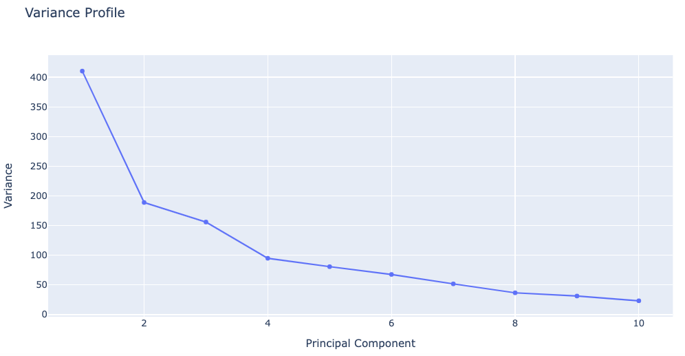
Plotting Variance Profile

The following plot shows the total variance of the trajectory and how it is distributed along the different eigenvectors. Variance appears in Å² and eigenvectors are shown according to eigenvalues descending order, the first one being the most important one and the last that with the lower contribution to variance. This graph indicates the size of the flexibility space (the higher the variance, the higher the flexibility) and how it is distributed in different modes.

with open(pcz_report, 'r') as f:
  pcz_info = json.load(f)
print(json.dumps(pcz_info, indent=2))

# Plotting Variance Profile
y = np.array(pcz_info['Eigen_Values'])
x = list(range(1,len(y)+1))

plotly.offline.init_notebook_mode(connected=True)

fig = {
    "data": [go.Scatter(x=x, y=y)],
    "layout": go.Layout(title="Variance Profile",
                        xaxis=dict(title = "Principal Component"),
                        yaxis=dict(title = "Variance")
                       )
}

plotly.offline.iplot(fig)

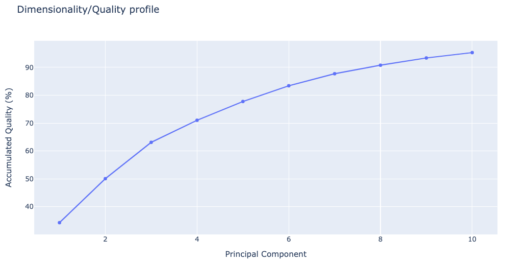
Plotting Dimensionality/quality profile

The following plot shows the percentage of explained variance for a given number of eigenvectors (quality) and the dimensionality of the sampled space. This graph indicates the complexity of the flexibility space, i.e. how many modes are necessary to explain the entire flexibility of the protein.

Note that this plot and the previous one provide physically-different information and that proteins might display a very complex pattern of flexibility (leading to large dimensionality) and at the same time be quite rigid (low variance), or have a large variance which can be fully explained by a very small number of modes.

# Plotting Dimensionality/quality profile
y = np.array(pcz_info['Eigen_Values_dimensionality_vs_total'])
x = list(range(1,len(y)+1))

plotly.offline.init_notebook_mode(connected=True)

fig = {
    "data": [go.Scatter(x=x, y=y)],
    "layout": go.Layout(title="Dimensionality/Quality profile",
                        xaxis=dict(title = "Principal Component"),
                        yaxis=dict(title = "Accumulated Quality (%)")
                       )
}

plotly.offline.iplot(fig)

PCA Eigenvectors & Eigenvalues

As stated above, the generated set of eigenvectors (the modes or the principal components) describe the nature of the deformation movements of the protein, whereas the eigenvalues indicate the stiffness associated to every mode. Inspection of the atomic components of eigenvalues associated to the most important eigenvectors helps to determine the contribution of different residues to the key essential deformations of the protein.

The pcz_evecs building block returns the atomic components of the eigenvalue associated to a given eigenvector.

Building Blocks used:

pcz_evecs from biobb_flexserv.pcasuite.pcz_evecs

from biobb_flexserv.pcasuite.pcz_evecs import pcz_evecs

pcz_evecs_report = pdbCode + "_pcz_evecs.json"

prop = {
    'eigenvector': 1
}

pcz_evecs( 
        input_pcz_path=concat_pcz,
        output_json_path=pcz_evecs_report,
        properties=prop)

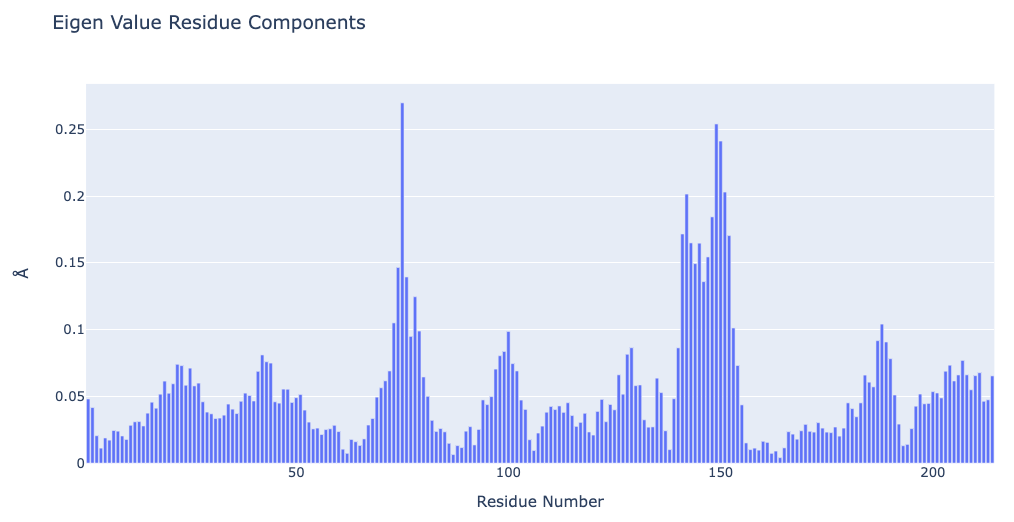
Plotting Eigenvalue Residue Components

Showing the contribution of different residues to the key essential deformations of the protein. The plot is displaying the residue contributions along the first principal component. The eigenvector property from the previous cell can be changed to explore the different principal components.

with open(pcz_evecs_report, 'r') as f:
  pcz_evecs_report_json = json.load(f)
print(json.dumps(pcz_evecs_report_json, indent=2))

# Plotting Eigen Value Residue Components
y = np.array(pcz_evecs_report_json['projs'])
x = list(range(1,len(y)+1))

plotly.offline.init_notebook_mode(connected=True)

fig = {
    "data": [go.Bar(x=x, y=y)],
    "layout": go.Layout(title="Eigen Value Residue Components",
                        xaxis=dict(title = "Residue Number"),
                        yaxis=dict(title = "\u00C5")
                       )
}

plotly.offline.iplot(fig)

Animate Principal Components

Motions described by the eigenvectors can be visualized by projecting the trajectory onto a given eigenvector and taking the 2 extreme projections and interpolating between them to create an animation. This type of visualization is extremely popular as it allows a graphical an easy way to identify the essential deformation movements in macromolecules.

The pcz_animate building block generates the animation of the macromolecule for a given eigenvector.

Building Blocks used:

pcz_animate from biobb_flexserv.pcasuite.pcz_animate

from biobb_flexserv.pcasuite.pcz_animate import pcz_animate

proj1 = pdbCode + "_pcz_proj1.crd"

prop = {
    'eigenvector': 1  # Try changing the eigenvector number!
}

pcz_animate( input_pcz_path=concat_pcz,
        output_crd_path=proj1,
        properties=prop)

Converting the generated ensemble (for visualization purposes)

Building Blocks used:

cpptraj_convert from biobb_analysis.ambertools.cpptraj_convert

from biobb_analysis.ambertools.cpptraj_convert import cpptraj_convert

proj1_dcd = pdbCode + '_pcz_proj1.dcd'

prop = {
    'format': 'dcd'
}

cpptraj_convert(input_top_path=prot_ca,
                input_traj_path=proj1,
                output_cpptraj_path=proj1_dcd,
                properties=prop)

Visualizing the generated ensemble (as a trajectory)

# Show trajectory
view = nglview.show_simpletraj(nglview.SimpletrajTrajectory(proj1_dcd, prot_ca), gui=True)
#view.add_representation(repr_type='spacefill', radius=0.7, selection='all')
view.add_representation(repr_type='surface', selection='all')
view.center()
view._remote_call('setSize', target='Widget', args=['','600px'])
view

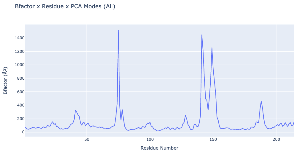
B-Factor x Principal Components

The B-factor is the standard measure of residue/atom flexibility. It is determined from the oscillations of a residue with respect to its equilibrium position:

B-factor profiles represent the distribution of residue harmonic oscillations. They can be compared with X-ray data, but caution is needed, since crystal lattice effects tend to rigidify exposed protein residues. Very large B-factors should be taken with caution since indicate very flexible residues that might display conformational changes along the trajectory, which is difficult to follow within the harmonic approximation implicit to B-factor analysis.

The generated PDB file can be used to plot an animation of the protein backbone coloured by the B-factor corresponding to the selected Principal Component. Such visualization makes easier to evaluate which region of the protein is involved in the movement.

The pcz_bfactor building block returns the B-factor values associated to a given eigenvector.

Building Blocks used:

pcz_bfactor from biobb_flexserv.pcasuite.pcz_bfactor

from biobb_flexserv.pcasuite.pcz_bfactor import pcz_bfactor

bfactor_all_dat = pdbCode + "_bfactor_all.dat"
bfactor_all_pdb = pdbCode + "_bfactor_all.pdb"

prop = {
    'eigenvector': 0,
    'pdb': True
}

pcz_bfactor( 
    input_pcz_path=concat_pcz,
    output_dat_path=bfactor_all_dat,
    output_pdb_path=bfactor_all_pdb,
    properties=prop
)

Plotting B-factors x Residue x PCA mode

# Plotting the B-factors x Residue x PCA mode
y = np.loadtxt(bfactor_all_dat)
x = list(range(1,len(y)+1))

plotly.offline.init_notebook_mode(connected=True)

fig = {
    "data": [go.Scatter(x=x, y=y)],
    "layout": go.Layout(title="Bfactor x Residue x PCA Modes (All)",
                        xaxis=dict(title = "Residue Number"),
                        yaxis=dict(title = "Bfactor (" + '\u00C5' +'\u00B2' + ")")
                       )
}

plotly.offline.iplot(fig)

Visualizing the B-factor along the first principal component

Visualizing the trajectory highlighting the residues with higher B-factor values, the most flexible residues of the protein.

# Show trajectory
view = nglview.show_simpletraj(nglview.SimpletrajTrajectory(proj1_dcd, bfactor_all_pdb))
view.add_representation(repr_type='spacefill', selection='all', colorScheme='bfactor')
view.add_representation(repr_type='tube', radius='0.4', selection='all', color='white')
view._remote_call('setSize', target='Widget', args=['','600px'])

stop = False
def loop(view):
    import time
    def do():
        while True and not stop:
            if view.frame == view.max_frame:
                direction = -1
            if view.frame == 0:
                direction = 1
            view.frame = view.frame + direction
            time.sleep(0.2)
    view._run_on_another_thread(do)
        
view.on_displayed(loop)

view._iplayer.children[0].disabled = True
view._iplayer.children[1].disabled = True

view

Hinge Points Prediction

Hinge point detection is a process to determine residues around which large protein movements are organized. Analysis implemented in the biobb_flexserv module can be performed using three different methodologies: B-Factor slope change method, Force constant method and Dynamic domain detection method.

The pcz_hinges building block computes the hinge points of the macromolecules associated to a given eigenvector.

Building Blocks used:

pcz_hinges from biobb_flexserv.pcasuite.pcz_hinges

from biobb_flexserv.pcasuite.pcz_hinges import pcz_hinges

hinges_bfactor_report = pdbCode + "_hinges_bfactor_report.json"
hinges_dyndom_report = pdbCode + "_hinges_dyndom_report.json"
hinges_fcte_report = pdbCode + "_hinges_fcte_report.json"

bfactor_method = "Bfactor_slope"
dyndom_method = "Dynamic_domain"
fcte_method = "Force_constant"

bfactor_prop = {
    'eigenvector': 0, # 0 = All modes
    'method': bfactor_method
}

dyndom_prop = {
    'eigenvector': 0, # 0 = All modes
    'method': dyndom_method
}

fcte_prop = {
    'eigenvector': 0, # 0 = All modes
    'method': fcte_method
}

pcz_hinges( 
        input_pcz_path=concat_pcz_gaussian,
        output_json_path=hinges_bfactor_report,
        properties=bfactor_prop
)

pcz_hinges( 
        input_pcz_path=concat_pcz_gaussian,
        output_json_path=hinges_dyndom_report,
        properties=dyndom_prop
)

pcz_hinges( 
        input_pcz_path=concat_pcz_gaussian,
        output_json_path=hinges_fcte_report,
        properties=fcte_prop
)

Visualizing the hinge points predictions

with open(hinges_bfactor_report, 'r') as f:
  hinges_bfactor = json.load(f)
print(json.dumps(hinges_bfactor, indent=2))

with open(hinges_dyndom_report, 'r') as f:
  hinges_dyndom = json.load(f)
print(json.dumps(hinges_dyndom, indent=2))

with open(hinges_fcte_report, 'r') as f:
  hinges_fcte = json.load(f)
print(json.dumps(hinges_fcte, indent=2))

# Show trajectory
view1 = nglview.show_simpletraj(nglview.SimpletrajTrajectory(proj1_dcd, bfactor_all_pdb), gui=True)
view1.add_representation(repr_type='surface', selection=hinges_dyndom["clusters"][0]["residues"], color='red')
view1.add_representation(repr_type='surface', selection=hinges_dyndom["clusters"][1]["residues"], color='green')
#view1.add_representation(repr_type='surface', selection=hinges_dyndom["clusters"][2]["residues"], color='yellow')
#view1.add_representation(repr_type='surface', selection=hinges_dyndom["hinge_residues"], color='red')
view1._remote_call('setSize', target='Widget', args=['350px','350px'])
view1
view2 = nglview.show_simpletraj(nglview.SimpletrajTrajectory(proj1_dcd, bfactor_all_pdb), gui=True)
view2.add_representation(repr_type='surface', selection=hinges_bfactor["hinge_residues"], color='red')
view2._remote_call('setSize', target='Widget', args=['350px','350px'])
view2
view3 = nglview.show_simpletraj(nglview.SimpletrajTrajectory(proj1_dcd, bfactor_all_pdb), gui=True)
view3.add_representation(repr_type='surface', selection=str(hinges_fcte["hinge_residues"]), color='red')    
view3._remote_call('setSize', target='Widget', args=['350px','350px'])
view3
ipywidgets.HBox([view1, view2, view3])

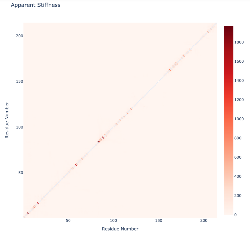
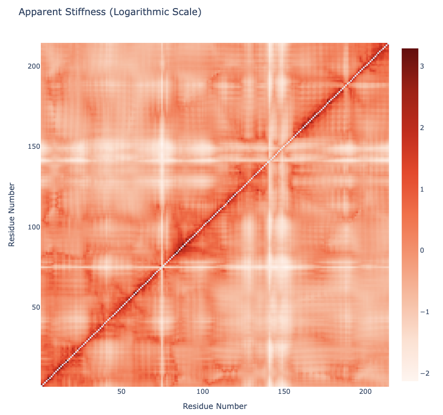
Apparent Stiffness

Stiffness is defined as the force-constant acting between two residues in the case of completely disconnected oscillators. The index helps to detect strong interactions between residues, which might indicate physically-intense direct contacts or strong chain-related interactions. Results are usually plot as a 2D NxN heatmap plot (with N being the number of residues).

The pcz_stiffness building block returns the stiffness force-constants associated to a given eigenvector.

Building Blocks used:

pcz_stiffness from biobb_flexserv.pcasuite.pcz_stiffness

from biobb_flexserv.pcasuite.pcz_stiffness import pcz_stiffness

stiffness_report = pdbCode + "_pcz_stiffness.json"

prop = {
    'eigenvector': 0 # 0 = All modes
}

pcz_stiffness( 
        input_pcz_path=concat_pcz,
        output_json_path=stiffness_report,
        properties=prop
)

Plotting the Apparent Stiffness matrix

with open(stiffness_report, 'r') as f:
  pcz_stiffness_report = json.load(f)
print(json.dumps(pcz_stiffness_report, indent=2))

y = np.array(pcz_stiffness_report['stiffness'])
x = list(range(1,len(y)))

plotly.offline.init_notebook_mode(connected=True)

fig = {
    "data": [go.Heatmap(x=x, y=x, z=y, type = 'heatmap', colorscale = 'reds')],
    "layout": go.Layout(title="Apparent Stiffness",
                        xaxis=dict(title = "Residue Number"),
                        yaxis=dict(title = "Residue Number"),
                        width=800, height=800
                       )
}

plotly.offline.iplot(fig)

Plotting the Apparent Stiffness matrix (Logarithmic Scale)

y = np.array(pcz_stiffness_report['stiffness_log'])
x = list(range(1,len(y)))

plotly.offline.init_notebook_mode(connected=True)

fig = {
    "data": [go.Heatmap(x=x, y=x, z=y, type = 'heatmap', colorscale = 'reds')],
    "layout": go.Layout(title="Apparent Stiffness (Logarithmic Scale)",
                        xaxis=dict(title = "Residue Number"),
                        yaxis=dict(title = "Residue Number"),
                        width=800, height=800
                       )
}

plotly.offline.iplot(fig)

Collectivity Index

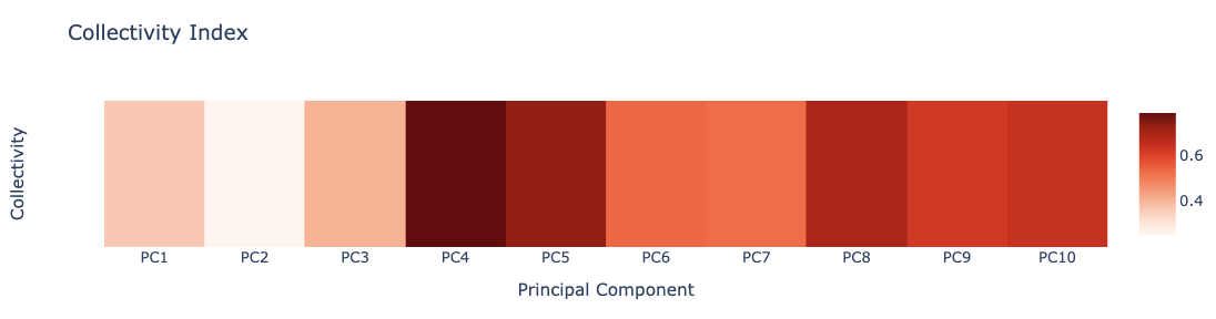
Collectivity index is a numerical measure of how many atoms are affected by a given mode (see the work by Rafael Brüschweiler: Collective protein dynamics and nuclear spin relaxation).

The pcz_collectivity building block returns the collectivity index of the macromolecule associated to a given eigenvector.

Building Blocks used:

pcz_collectivity from biobb_flexserv.pcasuite.pcz_collectivity

from biobb_flexserv.pcasuite.pcz_collectivity import pcz_collectivity

pcz_collectivity_report = pdbCode + "_pcz_collectivity.json"

prop = {
    'eigenvector':0 # 0 = All modes
}

pcz_collectivity( 
    input_pcz_path=concat_pcz,
    output_json_path=pcz_collectivity_report,
    properties=prop
)

Plotting the Collectivity indexes associated to the first 10 PCA modes

with open(pcz_collectivity_report, 'r') as f:
  pcz_collectivity_report_json = json.load(f)
print(json.dumps(pcz_collectivity_report_json, indent=2))

z = np.array(pcz_collectivity_report_json['collectivity'])
x = list(range(1,len(z)+1))
x = ["PC" + str(pc) for pc in x]

y = [""]

plotly.offline.init_notebook_mode(connected=True)

fig = {
    "data": [go.Heatmap(x=x, y=y, z=[z], type = 'heatmap', colorscale = 'reds')],
    "layout": go.Layout(title="Collectivity Index",
                        xaxis=dict(title = "Principal Component"),
                        yaxis=dict(title = "Collectivity"),
                        width=1000, height=300
                       )
}

plotly.offline.iplot(fig)

Questions & Comments

Questions, issues, suggestions and comments are really welcome!

GitHub issues:
- https://github.com/bioexcel/biobb
BioExcel forum:
- https://ask.bioexcel.eu/c/BioExcel-Building-Blocks-library

Conformational ensembles generation, data representation and visualization of predicted flexibility properties using BioExcel Building Blocks (biobb) and FlexDyn tools

Conformational landscape of native proteins

Settings

Biobb modules used

Auxiliary libraries used

Conda Installation and Launch

linux

macos

Pipeline steps

Input parameters

Fetching PDB structure

Selecting a model

Selecting a monomer

Visualizing the protein

Generating the reduced (coarse-grained) structure (backbone)

Visualizing the protein

Generating the reduced (coarse-grained) structure (alpha carbons)

Visualizing the protein

Conformational Ensemble Generation

CONCOORD

Visualizing the generated ensemble

RMSd distribution of the generated ensemble

Visualizing the RMSd distribution

Converting the generated ensemble (for visualization purposes)

Visualizing the generated ensemble (as a trajectory)

PRODY

RMSd distribution of the generated ensemble

Visualizing the RMSd distribution

Converting the generated ensemble (for visualization purposes)

Visualizing the generated ensemble (as a trajectory)

FLEXSERV

Brownian Dynamics (BD)

RMSd distribution of the generated ensemble

Visualizing the RMSd distribution

Fitting and converting the generated ensemble (for visualization purposes)

Visualizing the generated ensemble (as a trajectory)

Discrete Molecular Dynamics (DMD)

RMSd distribution of the generated ensemble

Visualizing the RMSd distribution

Fitting and converting the generated ensemble (for visualization purposes)

Visualizing the generated ensemble (as a trajectory)

Normal Mode Analysis (NMA)

RMSd distribution of the generated ensemble

Visualizing the RMSd distribution

Converting the generated ensemble (for visualization purposes)

Visualizing the generated ensemble (as a trajectory)

NOLB

RMSd distribution of the generated ensemble

Visualizing the RMSd distribution

Converting the generated ensemble (for visualization purposes)

Visualizing the generated ensemble (as a trajectory)

iMOD

RMSd distribution of the generated ensemble

Visualizing the RMSd distribution

Converting the generated ensemble (for visualization purposes)

Visualizing the generated ensemble (as a trajectory)

Meta-Trajectory & Clustering

Building the meta-trajectory

Clustering the meta-trajectory

Visualizing the generated ensemble (cluster)

Macromolecular Flexibility Analyses

Principal Component Analysis

Fitting and converting the generated ensemble (meta-trajectory) (for visualization purposes)

Computing the Principal Component Analysis (PCA)

Analysing the PCA report

Plotting Variance Profile

Plotting Dimensionality/quality profile

PCA Eigenvectors & Eigenvalues

Plotting Eigenvalue Residue Components

Animate Principal Components

Converting the generated ensemble (for visualization purposes)

Visualizing the generated ensemble (as a trajectory)

B-Factor x Principal Components

Plotting B-factors x Residue x PCA mode

Visualizing the B-factor along the first principal component

Hinge Points Prediction

Visualizing the hinge points predictions

Apparent Stiffness

Plotting the Apparent Stiffness matrix

Plotting the Apparent Stiffness matrix (Logarithmic Scale)